Phonged surfaces
Adding phong to surfaces
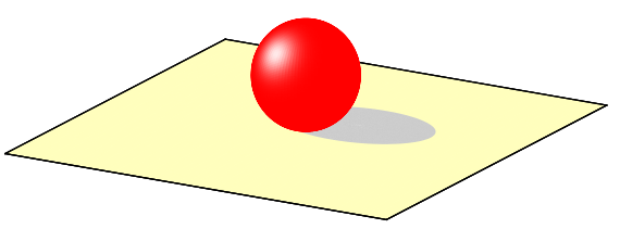
Another cool feature of a figure is its shininess, which is usually called phong, and gives the impression of three-dimensionality. I will show a relatively easy way to achieve this in gnuplot. With a few lines of code, we can produce a figure that looks like this one:
The only thing that is required is to note that in pm3d, colouring can be given specified by an arbitrary function in the fashion
splot 'some.dat' using 1:2:3:(f(...)) with pm3d
where some.dat contains our data, and f(...) denotes the function according to which we would like to colour the surface. You can read on this at the gnuplot central. The snag here is that this works only for data files where the surface is given as a x,y,z(x,y) triplet, but it will not do any good with functions. So, the first thing is to produce the surface data. This can easily be done by redirecting the plot to a table, which we will read back immediately. (If you recall, this is the trick that we used to add the figure a background with gradient in ...)
As in the figure above, we plotted a sphere, thus we write something like this:
set isosample 100,100
set parametric
set urange [0:1]
set vrange [0:1]
set table 'test.dat'
splot r*cos(2*pi*u)*sin(pi*v), r*sin(2*pi*u)*sin(pi*v), r*cos(pi*v)
unset table
This writes 10 000 points of a sphere to the file test.dat. Having created the surface, we have got to plot it, and give it the phong. We assume for the time being that the surface is red, and where light impinges on it, it is shining white. Therefore, we need a palette that runs from red to white, and it does not contain other colours. (This is a bit of a bumpy statement, but you get the meaning.) The one below will do: it is red, when the palette function's argument is 0, and glowing white, when the palette function takes the argument of 1.
set palette model RGB functions 1, gray, gray
Finally, we have to define the function itself. I am somewhat simple-minded, so I will just take a Gaussian function, and shift it in such a way that it takes the value 1, where I want to have the phong. Having these in mind, the complete code for the figure above reads as
reset
unset key
unset colorbox
set pm3d scansbackward
set isosample 100,100
unset ztics
unset xtics
unset ytics
set border 1+2+4+8

r = 1.0
x0 = -0.2*r
z0 = 0.7*r
y0 = -r*sqrt(1.0-x0*x0)

set parametric
set urange [0:1]
set vrange [0:1]
set table 'test.dat'
splot r*cos(2*pi*u)*sin(pi*v), r*sin(2*pi*u)*sin(pi*v), r*cos(pi*v)

unset table

set multiplot
set ticslevel 0

set xrange [-4*r:4*r]
set yrange [-4*r:4*r]
set zrange [-r:3.2*r]

# First, we draw the plane on which the sphere rests
set palette model RGB functions 1, 254.0/255.0, 189.0/255.0
splot -4*r+8*r*u, -4*r+8*r*v, -1 w pm3d

# Then, the shadow of the sphere
# This shall be an ellipse
set palette model RGB functions 0.8, 0.8, 0.8
splot (1.5*r*cos(2*pi*u)*v+r/sqrt(2.0)), (r*sin(2*pi*u)*v+r/sqrt(2.0)), -1 w pm

# And finally, the sphere itself
g(x) = x
b(x) = x
f(x,a,b) = exp(-(x-a)*(x-a)/b/b)
set palette model RGB functions 1, g(gray), b(gray)
splot 'test.dat' u 1:2:3:(f($3,z0,0.4)*f($1,x0,0.4)*f($2,y0,0.4)) w pm3d
unset multiplot
Note that we applied our Gaussian function in the last but one line, to give the phong at z=0.7, (3rd column in the data file) x=-0.2, (1st column in the data file), and y=0.98 (2nd column in the data file). The phong positions were defined somewhere at the beginning, as z0, x0, and y0. Also note that by changing the 3rd argument in the function, the tightness of the white spot can be modified: smaller value will give smaller spot, and vice versa.
We need the multiplot only because we plotted a plane on which the sphere rests, and we also drew a gray ellipse, which is supposed to represent the shadow of the sphere. If you do not need shadows and the like, the code is much simpler.
by Zoltán Vörös © 2009