Since it is somewhat hard to manage several web sites at the same time, I decided to give up this one. However, you can still check out my blog, where you should find plenty of interesting tricks on how to produce cool figures in gnuplot. The address is

Gnuplot tricks

Many say that it is impossible to produce a publication quality plot with gnuplot. I strongly believe that this assertion is simply wrong, and once you know what and how to do, gnuplot is just as good as it gets. Of course, one shouldn't forget that gnuplot is a plotting utility, and one won't have the conveniencies of FFT and the like, but this would be off the point. In the following pages, I explain a couple of tricks that will help you produce high-quality plots with gnuplot. While I understand the advantages of using a point-and-click type plotting utility (e.g. Origin under Windows, Kst, Grace, Labplot under Linux), there are certain things that are just much easier with gnuplot, once you get the hang of it.

Including unconventional symbols in a graph

So, you want to make a decent-looking, publication quality plot, with a couple of fancy symbols here and there. There are several ways to go.

Enhanced EPS

If all you need is a couple of greek symbols and the like, then the easiest route is to use the postscript terminal with the enhanced option, and simply enter the code for that particular letter. (postscript is not the only terminal that has an enhanced option, however, the degree to which those terminals are properly implemented is varying. Postscript works perfectly, while others don't.) So, you would write

gnuplot> set terminal postscript eps enhanced solid "Helvetica" 14

and then, if you want to have a label with an α in it, you write

gnuplot> set label 1 at graph 0.1, 0.1 "{/Symbol a}^2 = 12"

which, once you set the output and replot your graph, will place α²=12 at position (0.1,0.1) on your figure. You can find all available characters and their corresponding code in Dick Crawford's postscript guide While setting the characters is quite easy, the problem with this method is that the character set is somewhat limited (though, almost always enough), and that the relative placement of the characters must be done manually, through trial and error. E.g., you would have a hard time, if you tried to write an overhead vector on some symbol. If this is the case, then you should use the epslatex terminal of gnuplot. We cover this subject in the next paragraph.

Using the epslatex terminal

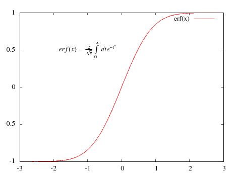
As always, first we have to set our terminal as

gnuplot> set terminal epslatex

At this point, we can set labels with any LaTeX symbols, the generated output will contain it properly. For the sake of example, we will plot the error function, and write its definition on the figure as follows:

gnuplot> set terminal epslatex
gnuplot> set xrange [-3:3]
gnuplot> set yrange [-1:1]
gnuplot> set label 1 at -2, 0.5 "$erf(x) = \\frac{2}{\\sqrt{\\pi}}\\int_0^x\\, dt e^{-t^2}$" centre
gnuplot> plot erf(x)

Note that we have crammed a lot of LaTeX commands in the label, enclosed by the two $ signs, to indicate that we are dealing with mathematical expressions. You might have to escape the instructions twice, so you will have \\frac{}{} etc. Now, if you set your output

gnuplot> set output 'errorf.tex'

and replot your graph, you will get two files. (At this point, I would also recommend re-setting the terminal, otherwise, there is no guarantee that gnuplot has closed both your output files, and this could create some trouble later on.) errorf.eps will contain the "visual" part of the graph, i.e., the axes, tics, points, lines, arrows and the like, while errorf.tex holds all the typographic elements. We then have got to combine these two by invoking LaTeX or pdflatex, depending on the exact route you would like to follow. The destination is the same in both cases. So, let us suppose for the moment that you want to work with postscript, and not with pdf. You should create a LaTeX file, which includes nothing but the file that we have just produced, errorf.tex.

\documentclass{article}
\usepackage{graphics}
\usepackage{nopageno}
\usepackage{txfonts}
\usepackage[usenames]{color}

\begin{document}
\begin{center}
  \input{errorf.tex}
\end{center}
\end{document}

You can read everything about epslatex in the gnuplot documentation. If you want to compile with pdflatex, first you have to convert the postscript file to pdf. In principle, one could use the pdf terminal of gnuplot, but I have had problems with that, and the end result is far from the expected. I would recommend using the eps terminal, and then converting the file by

ps2pdf -dEPSCrop error.eps error.pdf

Of course, this assumes that you have ghostview installe on your computer. By passing the -dEPSCrop argument to ps2pdf, we can retain the bounding box in the eps file, so the pdf graph won't be bigger. By this time, you should have something like this figure:

Plotting on top of a map

Sometimes you might want to have overlapping plots. The first thing that comes to my mind is a map, on which you would like to show a function that you have fitted to the peaks. An example is shown in the figure below. It works only with gnuplot 4.3 or later, though.
We will have to use multiplot. The standard way is to tell gnuplot what, where and in what size we want to plot, as in

set multiplot
set size 0.5, 1
set origin 0,0
plot sin(x)

set origin 0.5, 0
plot cos(x)
unset multiplot

The problem here is that when gnuplot determines how big the actual plot is going to be, it counts the borders, axis label, tics and so on in the size. So, in the example above, the width of 0.5 is the full with of one plot, and not the size of the plotting are, where the curve is shown. Thus, when putting two plots on top of each other, strange things might happen. The difficulty is that the second plot shouldn't contain axis labels, tics and so on. However, when one takes those off, there is no telling as to what the final size of that graph is going to be, and when they are on top of each other, there is a fair chance that they will be misaligned.
In order to alleviate the situation, we have to force gnuplot to allocate a certain amount of space for the curves, regardless the surroundings. We can do this with the command

set lmargin at screen 0.10
set rmargin at screen 0.85
set bmargin at screen 0.15
set tmargin at screen 0.95

where the four margins determine the white space on the left, right, bottom, and top, respectively. This won't work on gnuplot 4.2 or earlier. Once we have specified the margins, the rest is plain sailing. We plot both figures, and they will be aligned and top of each other.

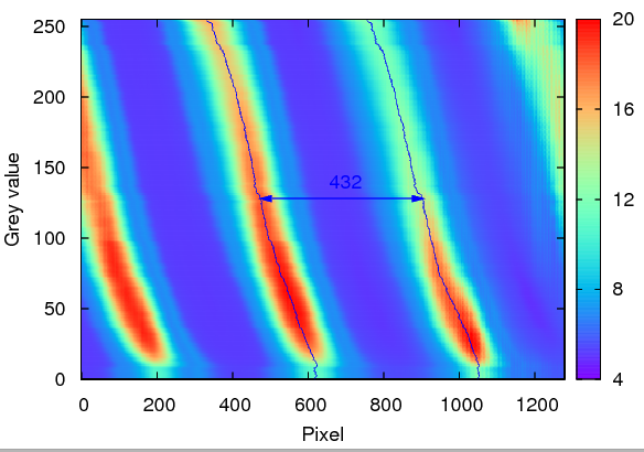
The gnuplot commands that produced this figure are

reset
set terminal postscript enhanced eps solid colour "Helvetica" 22
unset key
set multiplot
set lmargin at screen 0.10
set rmargin at screen 0.85
set bmargin at screen 0.15
set tmargin at screen 0.95
set pm3d map
set palette rgbformulae 33,13,10
set xrange [0:1279]
set yrange [0:255]
set cbrange [4e4:2e5]
set cbtics ("4" 4e4, "8" 8e4, "12" 12e4, "16" 16e4, "20" 20e4)
set xlabel 'Pixel'
set ylabel 'Grey value'
splot 'shiftimage.dat' mat
unset xtics
unset ytics
unset xlabel
unset ylabel
p 'peak1.dat' using 2:0 with lines lt 3, 'peak2.dat' using 2:0 with lines lt 3
unset multiplot

(Obviously, you should replace the file names with some appropriate ones.)
Incidentally, the same method can be used to plot things that are not on top of each other, but should still be aligned, as in the example below, where on the bottom, a horizontal, while on the left hand side, a vertical cut through the centre are shown.

And here is the code producing this graph

reset
set out 'multi.svg'
set term svg size 600,400 dynamic enhanced fname 'arial' fsize 11 butt solid
set multiplot
set lmargin screen 0.20
set rmargin screen 0.85
set bmargin screen 0.25
set tmargin screen 0.90

set pm3d map
set palette rgbformulae 33,13,10
set samples 50, 50
set isosamples 50, 50
set xrange [ -15.00 : 15.00 ]
set yrange [ -15.00 : 15.00 ]
set cbrange [ -0.250 : 1.000 ]
set cbtics -0.25,0.25,1

unset xtics
unset ytics
unset key

splot sin(sqrt(x**2+y**2))/sqrt(x**2+y**2)
unset pm3d
set lmargin screen 0.10
set rmargin screen 0.20
set ytics

set parametric
set dummy u,v
set view map

f(h) = sin(sqrt(h**2))/sqrt(h**2)

set urange [ -15.00 : 15.00 ]
set vrange [ -15.00 : 15.00 ]
set xrange [*:*]
set surface

splot f(u), u, 0 with lines lc rgb "green"

unset parametric
set lmargin screen 0.20
set rmargin screen 0.85
set bmargin screen 0.10
set tmargin screen 0.25
set xrange [ -15.00 : 15.00 ]
set yrange [ * : * ]
set xtics
unset ytics

plot sin(sqrt(x**2))/sqrt(x**2)
unset multiplot

Broken axes in gnuplot

A broken axis definitely comes handy, if part of a curve doesn't contain too much relevant information. Unfortunately, there is no easy way to do this in gnuplot. However, there is a work-around that can be applied in most situations. However, this method requires version 4.3 or later, so, if you don't have it, you should check it out on the development page.

For the sake of example, we will learn how to plot the cosine function in the [0:6π] interval with a break point at 2.5π and 4.5π.

First, we have to determine what is the ratio of the two parts of the figure. Since the first half is 2.5π long, while the second is 1.5π, we have to split the figure in a 2.5:1.5 ratio. I will choose 0.8 for the length of the whole figure (without the gap), so the first half will be 0.5 long, while the second 0.3. We then insert the first half in a multiplot, while keeping in mind that this part will have only three boundaries: left, bottom, and top. The border is defined as the sum of bottom (1), left (2), top (4), and right (8).

set multiplot
unset key
unset xlabel
set border 1+2+4
set lmargin at screen 0.10
set rmargin at screen 0.6
set bmargin at screen 0.15
set tmargin at screen 0.95

Then, we specify the range and the tic marks

set ytics -1,0.5,1 nomirror
set xrange [0:2.5*pi]
set xtics ("0" 0, "{/Symbol p}" pi, "2{/Symbol p}" 2*pi)

and we also add the two slanted tics that denote the broken axis. These will just be two arrows with no heads.

set arrow 1 from 2.5*pi-tiny, -1-tiny to 2.5*pi+tiny, -1+tiny nohead
set arrow 2 from 2.5*pi-tiny, 1-tiny to 2.5*pi+tiny, 1+tiny nohead

Now, that we are done with the outline of the first half, we plot the function, cosine in this case.

plot cos(x)

The second half is very similar, with some small differences: First, this graph will still have three boundaries, but on the bottom, right, and top. We also have to take off the vertical tics, and keep an eye on the position of the graph. Therefore, we have

unset ytics
set border 1+4+8
set key right
set lmargin at screen 0.63
set rmargin at screen 0.93
set bmargin at screen 0.15
set tmargin at screen 0.95
set label 1 'cos(x)' at screen 0.5, 0.05 centre
set xrange [4.5*pi:6*pi]
set xtics ("5{/Symbol p}" 5*pi, "6{/Symbol p}" 6*pi)
set arrow 1 from 4.5*pi-tiny, -1-tiny to 4.5*pi+tiny, -1+tiny nohead
set arrow 2 from 4.5*pi-tiny, 1-tiny to 4q.5*pi+tiny, 1+tiny nohead
plot cos(x)
unset multiplot

At the end of the plot, we closed the multiplot, and also added an xlabel, which is located at the centre of the whole graph. After setting the appropriate terminal, we get a figure that looks like this:

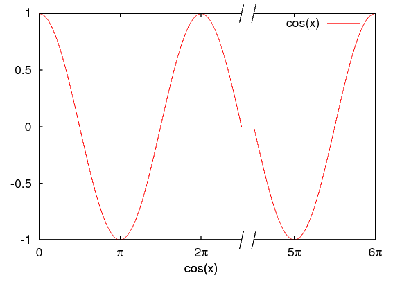
It's quite re-assuring that the cosine function has the same value at 2.5π and 4.5π. You would have never guessed, would you?

Plotting a histogram

From version 4.3, there is an option to plot data in a histogram, but this hasn't always been the case. However, there is a way to rectify the situation, using the smooth option. First, we have to define our bins, and then we have got to count the number of data points falling into each of the bins. The frequency specifier of the smooth option takes care of this, and we only have to determine into which bin a particular data point falls. The bin(x, width) function will do this; its working should be obvious. As an example, we take 10000 numbers normally distributed between 0 and 6, and plot their frequency. At the same time, we can also plot the cumulative frequency, which is another specifier of the smooth option.

unset key
set ylabel 'Frequency'
set y2label 'Cumulative frequency'
set y2tics 0,2e3,1e4
set ytics nomirror
set boxwidth 0.7 relative
set style fill solid 0.5
f(x) = a*exp(-(x-b)*(x-b)/c/c)
a=560.0
b=3.0
c = 1.0
bw = 0.1
bin(x,width)=width*floor(x/width)
plot 'gauss.dat' using (bin($1,bw)):(1.0) smooth frequency with boxes,\
'' using (bin($1,bw)):(1.0) smooth cumulative axis x1y2 w l lt 2 lw 2, \
f(x) w l lt 3 lw 2

Coloured axes

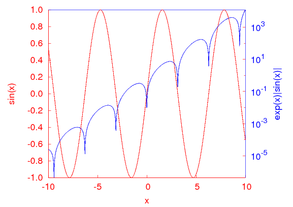
Sometimes you might need a left and a right vertical axis with different colours, to signify the scale that belongs to two curves shown on the graph. We will discuss an easy way to achieve this effect. Since we cannot set the colour of the axes one by one, we will do this in two steps. Let us suppose that the two axes should be red and blue.
First, we draw the border that is meant to be red. The command

set border 1+2 lt 1

sets the left and the bottom axis red, which is linetype 1. The top and the right axes are not drawn at this moment. We will plot sin(x) on the left axis. Then we draw two blue arrows without heads where the right and the top axes are supposed to be, as in

set arrow 1 from 10, -1 to 10, 1 nohead lt 3
set arrow 2 from -10,  1 to 10, 1 nohead lt 3

The function on the right axis will be exp(x)|sin(x)|, although it doesn't really matter. The rest of the code sets up the tics, label colours and the like. There is only one small thing worth looking at: when we specify the format of y2tics, we give it as format "10^{%T}", where %T is a format specifier, and it tells gnuplot to substitute the exponent of the 10-base value of the y2tics. Using specifiers like this, very nice results can be obtained. I will cover this subject in a later post.

reset
unset key
set border 1+2 lt 1
set y2tics 1e-5, 1e2, 1e5 textcolor rgb "blue" format "10^{%T}"
set ytics nomirror format "%.1f"
set xtics nomirror
set xlabel 'x' textcolor rgb "red"
set ylabel 'sin(x)' textcolor rgb "red"
set y2label 'exp(x)|sin(x)|' textcolor rgb "blue"
set log y2
set arrow 1 from 10, -1 to 10, 1 nohead lt 3
set arrow 2 from -10,  1 to 10, 1 nohead lt 3
set sample 1000
plot sin(x) with lines lt 1, exp(x)*abs(sin(x)) with lines lt 3 axis x1y2

After plotting the two functions, we would get a graph like this:

If the colour of the tics on y2 still bothers you, you can change it by tampering with the eps file.