Broken axes

We will now look at a different method, which eliminates these problems, and which requires very little human intervention. There is another method in gnuplot 4.3 (still in development), but I do not think that it would offer any advantages over this one. If you are interested, you can read about the details in my blog.

So, we would like to have something like this graph:

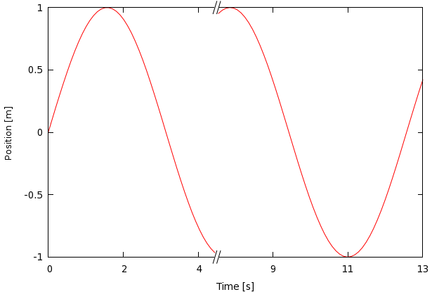
(This is just a sin function, broken at 4.5, and for the right hand side, displaced by 3). The recipe that we are going to follow takes only a couple of lines, and it runs as follows.

reset
A=4.5;	# This is where the break point is located  
B=3.0;	# This is how much is cut out of the graph 
C=0;		# The lower limit of the graph 
D=13;		# The upper limit (with the cut-out) of the graph 
E1=-1;	# The min of the y range
E2=1;		# The max of the y range
eps=0.05*(E2-E1)
eps2=0.005*(D-B-C)
 
f(x) = (xA?1:1/0)
h(x) = (x
set xtics 0, 2, A

set xtics add (gprintf("%.0f", 6+B) 6)
set xtics add (gprintf("%.0f", 8+B) 8)
set xtics add (gprintf("%.0f", 10+B) 10)

set yrange [E1:E2]
set arrow 1 from A-eps2, E1 to A+eps2, E1 nohead lc rgb "#ffffff" front
set arrow 2 from A-eps2, E2 to A+eps2, E2 nohead lc rgb "#ffffff" front
set arrow 3 from A-eps-eps2, E1-eps to A+eps-eps2, E1+eps nohead front
set arrow 4 from A-eps+eps2, E1-eps to A+eps+eps2, E1+eps nohead front
set arrow 5 from A-eps-eps2, E2-eps to A+eps-eps2, E2+eps nohead front
set arrow 6 from A-eps+eps2, E2-eps to A+eps+eps2, E2+eps nohead front
plot [C:D] f(x)*sin(x) w l lt 1, g(x)*sin(h(x)) w l lt 1

The first several lines are just definitions: A is the position at which we want to break the line, B is the value by which the right hand side of the graph will be shifted, or, in other words, this is how much we cut out of the graph, when traversing the break point. C, D, E1, and E2 are just definitions for the x and y ranges, while eps and eps2 will be needed for the drawing of the slanted tics representing the discontinuity in the axes. By linking the definitions of eps and eps2 to xrange and yrange, we make sure that the lookout of the figure does not depend on the range we want to plot.

The first really important definition is that of f(x), g(x) and h(x), which are helper functions (green lines). In all three cases, we use the ternary operator that I discussed elsewhere. Basically, f(x) returns 1, if x is smaller than A, g(x) does just the opposite, while h(x) produces a shift of its argument, if x is larger than A.

Then we set the labels on the x axis (blue line in the code). But watch out: we do it only up to A, because the axis is going to be broken at A. In order to make up for the missing tic marks, we add them in the next three lines (red). We can save some work, and can eliminate the possibility of messing something up, if we ask gnuplot to compute the values for us; this is done by the string conversion function gprintf, and adding the converted string.

set xtics add (gprintf("%.0f", 10+B) 10)

The last bit is drawing the break points on the axis. In order to do so, we draw 6 arrows with no heads. Note that the first two arrows are white, and they serve as a beauty plaster: we put them on top of the axes, to give the impression that the axes are broken. Also note that since arrows are drawn earlier than axes and borders, we have got to explicitly instruct gnuplot to bring the arrows to the front of the figure. The last four line segments are slightly slanted, to give a more appealing look to the graph. Once we are done with the set up of the figure, we can plot the function. The only thing we have to keep in mind is that the right hand side should be shifted by B, which is done by calling h(x) in the argument of sin(x).

The procedure for the y axis is very similar, so I just dodge the discussion of that, and I won't elaborate on broken axes with logarithmic axes either, for it should be straightforward. The only thing one should keep in mind is that with logarithmic plots the additions and subtractions should be replaced by multiplications and divisions in the definitions of eps and eps2.

I should point out that you can easily change the angle of the last 4 arrows by multiplying the shift of the y coordinates of the end points by something, and it is just as easy to move them farther from each other, if you replace the definition of eps2. Modifying eps will change their length, but not their angle.

Incidentally, this is not the only way to produce a figure with broken axes. This should be all right for raster figures, but it might be a tad problematic for vector graphics, because even if we cover those segments of the axes, it might still partially be visible in the output. If that is the case, we can fix it by drawing the four parts of the two axes by hand, as shown in this script:

reset
A=4.5;	# This is where the break point is located  
B=3.0;	# This is how much is cut out of the graph 
C=0;		# The lower limit of the x axis 
D=13;		# The upper limit (with the cut-out) of the x axis 
E1=-1;	# The minimum of the y range
E2=1;		# The maximum of the y range
eps=0.05*(E2-E1)
eps2=0.005*(D-B-C)
f(x) = (x<A?1:1/0)
g(x) = (x>A?1:1/0)
h(x) = (x<A?x:x+B)
set xtics 0, 2, A
set xtics add (gprintf("%.0f", 6+B) 6)
set xtics add (gprintf("%.0f", 8+B) 8)
set xtics add (gprintf("%.0f", 10+B) 10)
f(x) = (x<A?1:1/0)
g(x) = (x>A?1:1/0)
h(x) = (x<A?x:x+B)
set xtics 0, 2, A
set xtics add (gprintf("%.0f", 6+B) 6)
set xtics add (gprintf("%.0f", 8+B) 8)
set xtics add (gprintf("%.0f", 10+B) 10)

set border 2+8
set yrange [E1:E2]
set arrow 3 from A-eps-eps2, E1-eps to A+eps-eps2, E1+eps nohead front
set arrow 4 from A-eps+eps2, E1-eps to A+eps+eps2, E1+eps nohead front
set arrow 5 from A-eps-eps2, E2-eps to A+eps-eps2, E2+eps nohead front
set arrow 6 from A-eps+eps2, E2-eps to A+eps+eps2, E2+eps nohead front

set arrow 7 from C, E1 to A-eps, E1 nohead front
set arrow 8 from A+eps, E1 to D-B, E1 nohead front
set arrow 9 from C, E2 to A-eps, E2 nohead front
set arrow 10 from A+eps, E2 to D-B, E2 nohead front

plot [C:D] f(x)*sin(x) w l lt 1, g(x)*sin(h(x)) w l lt 1

This is basically the same as the previous, with two small differences. The first is that we draw only the y axes, i.e., set the border as

set border 2+8

which will draw the left (2) and the right (8) hand side of the border box. The second difference is that we now have to draw two more straight lines, instead of the white arrows, we have to draw them from the minimum of the xrange to the break point, and from the the break point to the apparent maximum of the xrange.