Keys with shadow
Adding shadow to the key
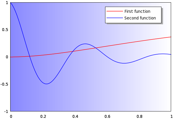
It changes the impression a graph can make by quite a lot, if it looks sort of three-dimensional. Even a tiny twist to the boring 2D lookout can make a difference, though it does not contain any new information. However, in a presentation, it is almost expected that one produces "exciting" graphs. In this section, we will discuss an easy way to add a slight shadow to the key on a graph, as if it were lifted from the plane of the curves. The resulting figure is
I believe the steps are quite straightforward, so I will not spend too much time on explaining every detail. Here is the script that we need
reset


xl=0; xh=1; yl=-1; yh=1;
eps=0.01;
rx=0.6; ry=0.8; kw=0.35; kh=0.15
lh=0.06; al=0.1


key1="First function"
key2="Second function"


set table 'shadowkey.dat'
splot [xl:xh] [yl:yh] x/(xh-xl)
unset table


set object 1 rect from graph rx,ry rto kw,kh fc rgb "#aaaaaa" fs solid 1.0 front lw 0
set object 2 rect from graph rx-eps,ry+eps rto kw,kh front fs empty
set label 1 at graph 1.1*al+rx, ry+2*lh key1 front
set label 2 at graph 1.1*al+rx, ry+lh key2 front
set arrow from graph rx, ry+2*lh rto al, 0 lt 1 lw 1.5 nohead front
set arrow from graph rx, ry+lh rto al, 0 lt 3 lw 1.5 nohead front


unset colorbox
unset key
set palette defined (0 "#8888ff", 1 "#ffffff")
plot [xl:xh] [yl:yh] 'shadowkey.dat' w ima, \
x*x*exp(-x) lw 1.5, cos(13*x)*exp(-3*x) lt 3 lw 1.5
We collect all variables at the beginning of the script, so that it will be easier to adapt it to any situations. The first four numbers define the xrange and the yrange. The next four numbers specify the position and the size of the key. We will have to make our own key, and the size of the key will depend on the particular terminal and font one uses. This is why it is handy to define them at the beginning of the script, so if you are not satisfied with the results, you can easily adjust both the position and the size. The next number (lh) gives the hight of one key line, while 'al' will be the length of the line which represents the curve. 'key1' and 'key2' are just two arbitrary strings, holding the text of the key.
The next three lines are necessary only if you want to draw the background gradient, but if you are happy with a white plot, you can skip this. I should also point out that the first four numbers that are needed for the xrange and yrange, are needed only because we have to "synchronise" the plot with its background, i.e., we have to make the background gradient exactly as big as the actual plot. If you don't want the gradient, you can drop these definitions, and you haven't got to specify the range in the plot either. This might be useful, when you don't know the plotting range beforehand, and want to let gnuplot calculate it for you.
The next step is to draw two rectangles in the front of the graph: one gray (this is going to be the shadow), and one white (this will contain the keys). Note that the rectangle in gray has no boundary, i.e., that is set to zero width. This might not take effect in all terminals. E.g., if you look at the pdf version of this figure, you will notice that there is a border to this rectangle. If this is the case, you can try to specify the colour of the border by adding the 'border' option, and a number, where the number represents the linetype. The downside is that in this case, you have got to use the defined line types, or define a line type which has the same colour as the body of the rectangle. Also note that we specify the coordinates in terms of the numbers we defined at the beginning, so both rectangles will change accordingly, if you change those numbers. This means that the white rectangle and its shadow will always be linked, and their relative placement is given by the variable 'eps'. When we are done with the white rectangle, we can place the text of the keys, and the two lines representing our plots. For this purpose we draw two arrows without heads, and with the linetypes that we will use for plotting the curves.
The final step is to actually draw the curves. Before that, we plot our file, 'shadowkey.dat', so the graph will have a background gradient. If you skipped these three lines writing the data file to disc, you should replace the plotting command by
plot [xl:xh] [yl:yh] x*x*exp(-x) lw 1.5, cos(13*x)*exp(-3*x) lt 3 lw 1.5
It should go without saying that in this case, you can also drop the palette definition, for it will not be used.
by Zoltán Vörös © 2009