Statistical patch to gnuplot
From the help: (For the complete documentation of the 'stats' command, follow the link.)
The `stats` command calculates basic summary statistics for a data set,
 displays them in human-readable form and (optionally) makes them available
 as gnuplot variables.

 Syntax:
       stats {<ranges>}
             {"<datafile>" {datafile-modifiers}}
             {[no]output} {variables[=prefix]}

 Permissible data file modifiers are `index`, `every`, and `using`, all of
 which behave exactly as for the `plot` command. Up to two columns can be
 specified with `using`, and inline transformations are available (same as
 for `plot`)...
The variables that are either defined or printed to the screen/file are the
following
	records : number of valid records found
	invalid : number of invalid records found
	blank   : number of blank lines found
	blocks  : number of data blocks in the file (separated by double blank lines)

	mean_*   : mean
	stddev_* : standard deviation
	sumx_*   : sum of all values
	sumx2_*  : sum of the squares of all values

	min_*         : minimal value
	min_pos_*     : position of the minimum value in file
	lo_quartile_* : lower quartile (defined at 25%)
	median_*      : median
	up_quartile_* : upper quartile (defined at 75%)
	max_*         : maximum value
	max_pos_*     : position of the maximum value in file
Examples
Here we would like to show a couple of examples as to how this patch can be used.
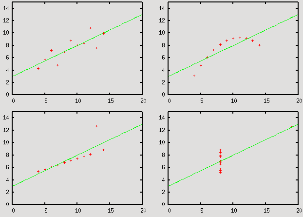
Linear regression
Simple linear regression (This particular case would basically be identical to the fit command.)unset key set xrange [0:20] set yrange [0:15] set multiplot layout 2,2 stat "anscombe" u 1:2 var noout plot "anscombe" u 1:2, slope*x + intercept stat "anscombe" u 3:4 var noout plot "anscombe" u 3:4, slope*x + intercept stat "anscombe" u 5:6 var noout plot "anscombe" u 5:6, slope*x + intercept stat "anscombe" u 7:8 var noout plot "anscombe" u 7:8, slope*x + intercept unset multiplotThe data file for this plot can be found here.
Using standard deviations, minimum, maximum and the like
# This first part up to 'set yrange [0:2]' is just to generate some data
set sample 50
set table 'stats1.dat'
plot [0:10] 0.5+rand(0)
unset table

set sample 200
set table 'stats2.dat'
plot [0:10] 0.5+rand(0)
unset table

set yrange [0:2]
unset key
set multiplot layout 2,2

# Plotting the minimum and maximum ranges with a shaded background
stats 'stats2.dat' u 1:2 var
set label 1 gprintf("Minimum = %g", min_y) at 2, min_y-0.2
set label 2 gprintf("Maximum = %g", max_y) at 2, max_y+0.2
plot min_y with filledcurves y1=mean_y lt 1 lc rgb "#bbbbdd", \
max_y with filledcurves y1=mean_y lt 1 lc rgb "#bbddbb", \
'stats2.dat' u 1:2 w p pt 7 lt 1 ps 1

# Plotting the range of the standard deviation  with a shaded background
stats 'stats2.dat' u 1:2 var
set label 1 gprintf("Mean = %g", mean_y) at 2, min_y-0.15
set label 2 gprintf("Sigma = %g", stddev_y) at 2, min_y-0.3
plot mean_y-stddev_y with filledcurves y1=mean_y+stddev_y lt 1 lc rgb "#bbbbdd", \
mean_y w l lt 3, 'stats2.dat' u 1:2 w p pt 7 lt 1 ps 1

# Removing points based on the standard deviation
stats 'stats2.dat' u 1:2 var
set label 1 gprintf("Mean = %g", mean_y) at 2, min_y-0.15
set label 2 gprintf("Sigma = %g", stddev_y) at 2, min_y-0.3
plot mean_y w l lt 3, mean_y+stddev_y w l lt 3, mean_y-stddev_y w l lt 3, \
'stats2.dat' u 1:(abs($2-mean_y) < stddev_y ? $2 : 1/0) w p pt 7 lt 1 ps 1

# Automatically adding an arrow at a position that depends on the min/max
stats 'stats1.dat' u 1:2 var
stats 'stats1.dat' u 1:2 every ::(min_pos_y-1)::(min_pos_y-1) var=min
stats 'stats1.dat' u 1:2 every ::(max_pos_y-1)::(max_pos_y-1) var=max
set arrow 1 from minmin_x, minmin_y-0.2 to minmin_x, minmin_y-0.02 lw 0.5
set arrow 2 from maxmax_x, maxmax_y+0.2 to maxmax_x, maxmax_y+0.02 lw 0.5
set label 1 'Minimum' at minmin_x, minmin_y-0.3 centre
set label 2 'Maximum' at maxmax_x, maxmax_y+0.3 centre
plot 'stats1.dat' u 1:2 w p pt 6

unset multiplot
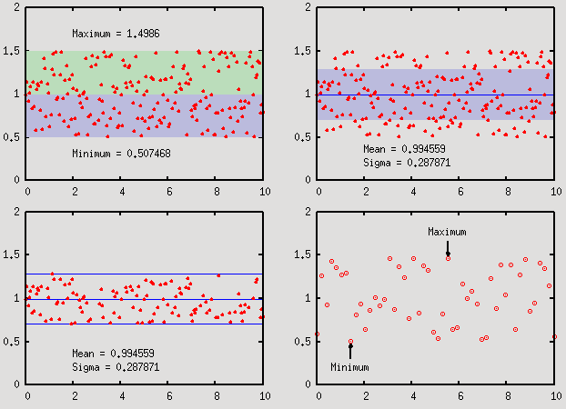
The first plot simply highlights the yrange of the data file, between its minimum and
maximum. The second plot shows the standard deviation, the third one plots only those
points that fall in the range of sigma around the mean, and in the fourth one, we place
arrows and labels positioned based on the statistical properties of the data set.
Note that in the fourth stats command, the every keyword has been used to specify the data
range, just as in the case of plot. In this particular case, we use it to pull out a single
value (the value of the x position) at the minimum or maximum.
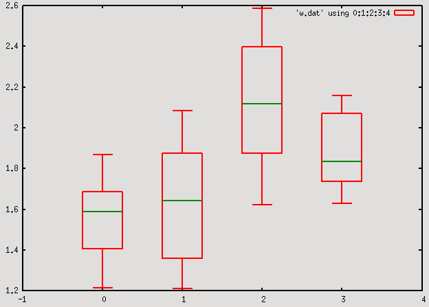
Whisker-and-box plots
# Again, the first part, up to 'unset table' is to generate data
set samples 50
set table 'whisker.dat'
a = 1.0+rand(0); b=0.5+rand(0)*0.5
p a+rand(0)*b
a = 1.0+rand(0); b=0.5+rand(0)*0.5
p a+rand(0)*b
a = 1.0+rand(0); b=0.5+rand(0)*0.5
p a+rand(0)*b
a = 1.0+rand(0); b=0.5+rand(0)*0.5
p a+rand(0)*b
unset table

set print 'w.dat'
stats 'whisker.dat' u 2 i 0 var noout
print lo_quartile_x, min_x, max_x, up_quartile_x, median_x
stats 'whisker.dat' u 2 i 1 var noout
print lo_quartile_x, min_x, max_x, up_quartile_x, median_x
stats 'whisker.dat' u 2 i 2 var noout
print lo_quartile_x, min_x, max_x, up_quartile_x, median_x
stats 'whisker.dat' u 2 i 3 var noout
print lo_quartile_x, min_x, max_x, up_quartile_x, median_x
set print

set xrange [-1:4]
set boxwidth 0.5
plot 'w.dat' using 0:1:2:3:4 with candlesticks whiskerbars 0.5 lw 2, \
'' using 0:5:5:5:5 with candlesticks notitle lw 2 lc rgb "#008800"
Here note that the index keyword has been used to specify the data block that we want to process.