Basic data analysis

Plotting the recession - some basic data analysis with gnuplot

In this section, I would like to discuss how we can do some very rudimentary data analysis, using gnuplot. Of course, if you want to analyse your data, then you can either use a dedicated script, written in a far better-fit language, e.g., in Perl or in gawk, or you can do the whole thing in a tabular environment, using Excel or Origin, or Grace, or Labplot. (Although, if you do that, then why would you be using gnuplot in the first place?) And I have also read somewhere that gnuplot conforms with the Unix philosophy, "one task - one tool", and we should not do any data processing with it. Now, there are at least two problems that I see with this approach: one is that some data analysis are really simple, and it is not clear, why one should use a separate tool for that. Furthermore, it will always cause some trouble (at least, in my experience) when the data analysis is not done from gnuplot, for one can never be sure how and on which version of the analysed data file the figure was based. And pipes can only be used on Linux/Unix-type systems, thus, the platform independence of gnuplot is lost. But more importantly, and if we are at the "philosophy" anyway, it is completely unclear (at least, to me) what constitutes plotting: just placing the curves, points and dots on an empty canvas, and writing a couple of labels for the axes, or this <it>and</it> the choice of the curves, points and dots, and "cleaning" up the data. The problem is that one can in most cases decide what to do with erroneous points and the like only when it is already plotted and shown. So, if that is the case, why should we sequester data analysis from the plotting? Are they not the two complementing parts of the very same procedure?

So, these are my reasons for doing data processing in gnuplot. However, the main motivations are not these only. I will use the same method in making automated generation of pie charts and bargraphs, which we could not do in gnuplot by other means. By the way, if you look at some of the demo scripts of gnuplot 4.3, you will immediately realise that the developers of gnuplot have already parted with the idea of "one task - one tool", and that there are ways of performing some simple analysis as the data are read in.

The kind of data processing we will do today requires a "recursive" access to data points, in particular, I will demonstrate how we can calculate the derivative and the integral of a series of data points. Calculating the derivative and integral of an analytic function is trivial, even if you do not have the analytical answer: for the derivative, you can simply plot f(x+dx)-f(x), where dx is just some pre-defined number, and for the integral you can apply a recursive scheme, detailed on the gnuplot demo site. But they work on known functions, and we would like to calculate something based on "measured" data. For this, I will take the weekly oil price of this year, which you can download from the link. Let us suppose that we plot the oil price, but we also want to highlight the time intervals where the price is dropping. This requires us to calculate the derivative at each point (In this particular case, we could get away just by comparing the value and the next, but we have got to get access to the values anyway, and we would get it by fitting a linear function, whose linear coefficient gives the derivative. So, for better of worse, I will just stick with the derivative.)

For a starter, let us see our two scripts! As I have already pointed out, we will have to walk through the values, one by one, so we will need a <it>for</it> loop, which means two scripts: a "master", and one that we call repeatedly.

reset
unset key
A=0; sa=1; sb=0; integ=0.0
f(x) = a*x+b
g(x) = (x>0?GPVAL_Y_MIN:GPVAL_Y_MAX)
set xlabel 'Time [weeks]'
set ylabel 'Crude oil price [$]'
set grid front
unset grid
p 'oil.dat' u 0:8

xmax = GPVAL_DATA_X_MAX

set print 'oild.dat' append
l 'derint_r.gnu'
set print

plot 'oild.dat' u 1:(g($2)) w filledcurve lc rgb "#eeeeee", 'oil.dat' u 0:8 w l

and our 'for' loop, that we call 'derint_r.gnu'

a=1.0; b=40.0
fit [A:A+1] f(x) 'oil.dat' u 0:8 via a, b
integ = integ+(a*A+b+a*(A+1)+b)/2.0
if(sa*a<0) print A, sa, sb, integ; print A, a, b, integ; sa=a; sb=b
if(sa*a>0) print A, a, b, integ; sa=a; sb=b
A=A+1
if(A<xmax) reread

The first part of the main script should be clear: we set up the style of our figure, and do a dummy plot to learn something about our data file, oil.dat. f(x) is our linear function, while g(x) is just a helper, whose role will become evident a bit later. The only really odd thing is in the two lines where we set a grid, and then immediately after that, unset it. The reason for that is that by sending the grid to front, we send the tics to the front, too. Since we do not actually need the grids, we can unset it. In this way, we can push the tics to the front of the plot, so that it will not be covered by the gray rectangles.

Having set up the plot, we call derint_r.gnu xmax times. So, what is in derint_r.gnu? We simply fit our linear function over a range that contains only two points, and we step through the whole file by moving those two points by one in each call to the loop. Then we calculate the integral by adding the area of the next trapezium, and then depending on whether the sign of the derivative, a, is different to the previous one, we print out the results once (if the signs are identical), or twice (if they are different). This distinction is necessary because we want to plot rectangles where the derivative is negative. After we are done with the data processing, we close our new file by setting the print, and plot the results, to get the following figure

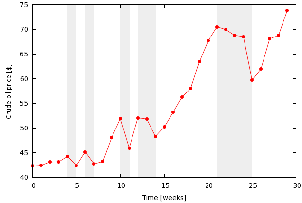
Note that in the plotting, we called the function g(x), which takes on the value of the minimum of the yrange, if the argument is negative (the price is dropping), while returns the maximum of the yrange otherwise. Of course, there are many things that we could do to improve the image, but I wanted only to demonstrate how we can do the data processing part.