Wall charts

In this section, I would like to discuss how to make a wall chart with gnuplot. In the first part, we will see how to do this, when we have a function to plot, while in the second one, I will show how we can manage this, when a data file is given.

Plotting a known function

There is a simpler version of wall charts, the so-called fence plot, that you can find on gnuplot's surface demo page, and in the first part, we will build on this. By the end of our adventure, we will have produced this graph:

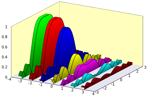
So, let us see what is to be done! First, I will just give the gnu script, and then discuss segments of it.

reset
A = 4
B = 3
C = 1
unset key
unset colorbox
f(x,y) = abs(sin(x*x+y*y)/(x*x+y*y)) # We plot this function
set isosample 2, 30
set parametric
set urange [-B:B]
set vrange [0:1]
set xrange [-A:A]
set yrange [-B:B]
set zrange [0:C]
set ticslevel 0 # We need this, in order to shift the 0 of the z axis
dx = 0.3 # Thickness of the walls
set multiplot
set border 1+2+4+8+16+32+64+256+512
# Plot the "background" first
set palette model RGB functions 0.9, 0.9,0.95
splot -A+2*A*v, B*u,0 w pm3d
unset border; unset xtics; unset ytics; unset ztics
set palette model RGB functions 1, 254.0/255.0, 189.0/255.0
splot -A, B*u, C*v w pm3d, A*u, B, C*v w pm3d
x0 = -A+1
y0 = 0.0
set palette model RGB functions 0, gray/2+0.5, 0.0
splot x0-dx, u, f(u,y0) w l lt -1 lw 0.2, \
x0-dx*v, u, f(u,y0) w pm3d,\
x0, u, f(u,y0)*v with pm3d, \
x0, u, f(u,y0) w l lt -1 lw 0.2
x0 = x0+1
y0 = y0+0.5
set palette model RGB functions gray/2+0.5, 0.0, 0.0
splot x0-dx, u, f(u,y0) w l lt -1 lw 0.2, \
x0-dx*v, u, f(u,y0) w pm3d,\
x0, u, f(u,y0)*v with pm3d, \
x0, u, f(u,y0) w l lt -1 lw 0.2
x0 = x0+1
y0 = y0+0.5
set palette model RGB functions 0, 0, gray/2+0.5
splot x0-dx, u, f(u,y0) w l lt -1 lw 0.2, \
x0-dx*v, u, f(u,y0) w pm3d,\
x0, u, f(u,y0)*v with pm3d, \
x0, u, f(u,y0) w l lt -1 lw 0.2
x0 = x0+1
y0 = y0+0.5
set palette model RGB functions gray/2+0.5, gray/2+0.5, 0
splot x0-dx, u, f(u,y0) w l lt -1 lw 0.2, \
x0-dx*v, u, f(u,y0) w pm3d,\
x0, u, f(u,y0)*v with pm3d, \
x0, u, f(u,y0) w l lt -1 lw 0.2
x0 = x0+1
y0 = y0+0.5
set palette model RGB functions gray/2+0.5, 0, gray/2+0.5
splot x0-dx, u, f(u,y0) w l lt -1 lw 0.2, \
x0-dx*v, u, f(u,y0) w pm3d,\
x0, u, f(u,y0)*v with pm3d, \
x0, u, f(u,y0) w l lt -1 lw 0.2
x0 = x0+1
y0 = y0+0.5
set palette model RGB functions 0, gray/2+0.5, gray/2+0.5
splot x0-dx, u, f(u,y0) w l lt -1 lw 0.2, \
x0-dx*v, u, f(u,y0) w pm3d,\
x0, u, f(u,y0)*v with pm3d, \
x0, u, f(u,y0) w l lt -1 lw 0.2
x0 = x0+1
y0 = y0+0.5
set palette model RGB functions gray/3+0.3, 0, 0
splot x0-dx, u, f(u,y0) w l lt -1 lw 0.2, \
x0-dx*v, u, f(u,y0) w pm3d,\
x0, u, f(u,y0)*v with pm3d, \
x0, u, f(u,y0) w l lt -1 lw 0.2
unset multiplot

In the first part, we set up the plotting ranges and the function that we want to plot. Note that in order to shift the 0 of the z axis, we have explicitly got to call 'set ticslevel 0'. We can also notice that in the graph above, the top surface is invariant under translations along the x axis, therefore, we can reduce the sampling frequency in that direction. This shouldn't matter, if you make a bitmap file, but it is going to save you a lot of space, if you produce a vector output, e.g., eps or svg.

Having finished the set-up, we plot the background, i.e., we will just plot three planes, the x-y (this one in gray), the y-z, and the x-z. These latter ones are in yellow. We set the colours in the colour scheme of the appropriate plots, by calling 'set palette model RGB functions 0.9, 0.9,0.95', which produces a shade of gray with a bluish tinge. Also note that we unset the border, and the tics immediately after the first plot. The reason for this is that in this way, we can avoid having gnuplot plot the axes and the tics more than once. By the way, before the first plot, we set the border as 'set border 1+2+4+8+16+32+64+256+512', which draws the frame along all, but the three front edges. You can learn how to set the border by reading the output of the command

?border

After having plotted the 'background' of the graph, we plot the first wall. In order to give it some 3D lookout, we have got to plot actually 4 different things: the vertical wall facing us, the top of the body, and the two relevant edges. The first two plots are surfaces, while the latter two are lines, so we call appropriate modifiers to splot, namely, 'with pm3d' and 'with lines'. We have also got to specify the colour of the walls, which we did by issuing 'set palette model RGB functions 0, gray/2+0.5, 0.0' before the first plot. The rest of the script is nothing but the repetition of these seven lines. Letting x0 = x0 + 1, we move the walls along the x axis, while letting y0 = y0 + 0.5, we plot a new function each time. Since we want each wall to have a different colour, we also need to change the palette in each step.

There are two remarks that we can make. The first is that the order of plotting the wall, the top and the two edges depends on the view, so don't be surprised, if you rotate the figure and all of a sudden, it looks messy! The second comment is that you can easily 'close' the graphs, by adding one parametric plot to each of the walls, which would be something like this:

x0-dx*v, -B, f(x0,-B)*(B+u)/(2*B) w pm3d

Plotting data

In most cases, one wants to plot data of a measurement or simulation, i.e., something that was produced not in gnuplot, but by some other means. In those cases, we cannot follow the procedure outlined above. But nothing is lost! We will see that we quite a few different graph types can be made using the same recipe. I will draw on the discussion in the section on ribbon charts, so before proceeding, you should cast at least a cursory glance at that.

Before we turn to the complete chart, first we should see how we can plot just one single "plane", taken the values from the file. For the sake of simplicity, I will use ribbon.dat, given in the section on ribbon charts.

If you recall, our data file, after some processing in gnuplot, looked like this (well, at least, the first column)

#Surface 0 of 1 surfaces

#IsoCurve 0, 3 points
#x y z type
0  13  0.901743 i
1  13  0.901743 i
2  13  0 i

#IsoCurve 1, 3 points
#x y z type
0  12  0.860648 i
1  12  0.860648 i
2  12  0 i
...

This is what we called rib2.dat. We used the every keyword of splot to single out the first (0) and second (1) line in gnuplot. Now, what would happen, if we plotted the second and third lines? We would get a single "plane", standing vertically, and having a "shape" given by the z values, as in this figure:

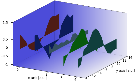
Just for the record, our plot is produced by these three lines in ribbon_r.gnu

r=rand(0); g=rand(0); b=rand(0)
set palette model RGB defined (0 r/cm g/cm b/cm, 1 r/cm g/cm b/cm)
splot 'rib2.dat' every ::1::2 u (A-1):2:3 w pm3d

i.e., we restrict the x values to A-1, and plot the second and third columns of the second and third records in each block. (Remember that the numbering of the records begins with 0!) The figure is almost OK, with the tiny glitch that the negative values are plotted "downwards", i.e., the reference line is 0. We can fix this with the helper function

zr(x) = (x==0?zmin:x)

which returns the minimum of the zrange, if the z value is smaller, than 0, otherwise it returns z. So, by modifying the plot as

r=rand(0); g=rand(0); b=rand(0)
set palette model RGB defined (0 r/cm g/cm b/cm, 1 r/cm g/cm b/cm)
splot 'rib2.dat' every ::1::2 u (A-1):2:(zr($3)) w pm3d

we get

Remember that, since we use a random number to determine the RGB values, the colour scheme of the plot will be different after each call of the script, and this is why the plot looks a bit different to the previous one. Nevertheless, the point is not this, but that the plots go up from the bottom of the graph to the corresponding z values. If you are satisfied with this, you can stop here, there is nothing more to it. However, we could turn what we have into a "real" wall chart by adding a "roof" to the walls. All it takes is four extra lines in our for loop, which will now look like this (this is wall_r.gnu for reference)

A=A+1
set table 'rib.dat'
plot filename u A:A
unset table

set table 'rib2.dat'
splot 'rib.dat' mat
unset table

r=rand(0); g=rand(0); b=rand(0)
set palette model RGB defined (0 r/cm/cm g/cm/cm b/cm/cm, 1 r/cm/cm g/cm/cm b/cm/cm)
splot 'rib2.dat' every ::1::2 u (A-1):2:(zr($3)):3 w pm3d

set palette model RGB defined (0 r g b, 1 r g b)
splot 'rib2.dat' every ::0::1 u (A-1+B*$1):2:3 w pm3d

set palette model RGB defined (0 r/cm g/cm b/cm, 1 r/cm g/cm b/cm)
splot 'rib2.dat' every ::1::2 u (A-1+B):2:(zr($3)):3 w pm3d

if(A<C) reread

Note that we plot the same file, rib2.dat, thrice, each time with a different shade of the same colour: first with the darkest, and this is the plane farthest from the viewer, then the roof of the walls, i.e., the ribbons, with the lightest, and finally, the front plane of the walls with a medium shade. The main script reads as follows

reset
filename="ribbon.dat"
mult=1.2; cm=1.4
A=0; B=0.3;
set xlabel 'x axis [a.u.]'; set ylabel 'y axis [a.u.]';
set ticslevel 0
unset key; unset colorbox
set tics out nomirror
set border 1+2+4+8+16+32+64+256+512 back
mini(x)=(x<0?x*mult:x/mult)>0?x*mult:x/mult)
zr(x) = (x==0?zmin:x)

set isosample 100, 3
set xrange [0:1]; set yrange [0:1]
set table 'bg.dat'
splot x
unset table; set xrange [*:*]; set yrange [*:*]

splot filename mat
C=GPVAL_DATA_X_MAX+1
ymax = GPVAL_DATA_Y_MAX+1
zmin = mini(GPVAL_DATA_Z_MIN)
zmax = maxi(GPVAL_DATA_Z_MAX)
set xrange [-0.5:C-0.5]
set yrange [0:ymax]
set zrange [zmin:zmax]
set cbrange [0:1]

set multiplot
set palette model RGB defined (0 0.3 0.3 0.85, 1 0.9 0.9 0.95)
splot 'bg.dat' u ($1*C-0.5):($2*ymax):(zmin):3 w pm3d, \
'' u ($1*C-0.5):(ymax):(1.9999*$2*(zmax-zmin)+zmin):3 w pm3d, \
'' u (-0.5):($1*ymax):(1.9999*$2*(zmax-zmin)+zmin):(0) w pm3d
set cbrange [zmin:zmax]

unset border; unset tics; unset xlabel; unset ylabel; unset zlabel

l 'wall_r.gnu'

unset multiplot

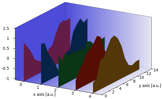
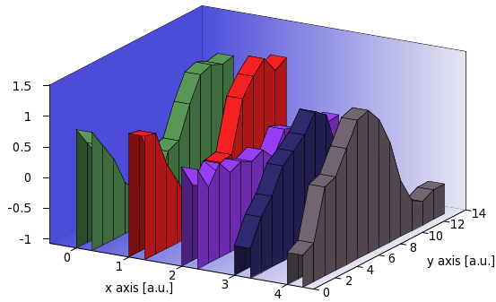
This is identical to ribbon.gnu, with the exception of the definition of the helper function zr(x). The resulting figure looks like this one

There are two more things that we could do with this graph: One is that we can add a grid to the surfaces by adding these three lines to our for loop

set style line 1 lt -1 lw 0.5 ps 0
set pm3d implicit at s
set pm3d depthorder hidden3d 1

(Or, we could add this to our main script, but only after plotting the background, otherwise, that will be gridded, too.) By doing so, we get the following figure

The second is that instead of drawing the back plane of the wall, we could add a front plane, thereby "closing" the volume. We do this by replacing the first plot command in our for loop by

splot 'rib2.dat' every ::0:(ymax-2):1:(ymax-1) u (A-1+B*$1):(0):(zz($2,$3)) w pm3d

and adding the helper function

zz(x,y) = (x==1?zmin:y)

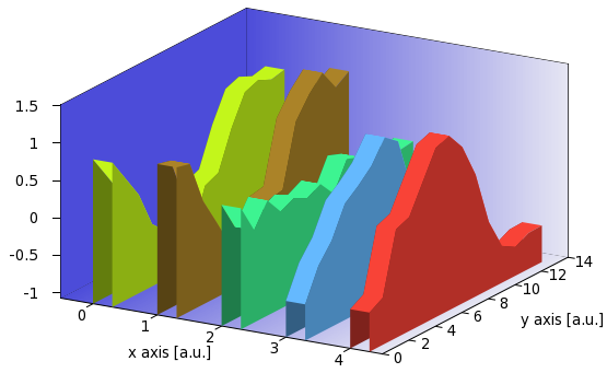
to the main script. What the plotting command does is to take only the last two blocks, and choose only the first and second records. The last two blocks will have 1 and 0 in the second column, so we use that and the helper function to determine which z value we want to pick to draw our rectangle in the front. Of course, you should plot the front plane after you plotted the ribbon on the top, otherwise, parts of it might be covered. Once you do that, you get the following image

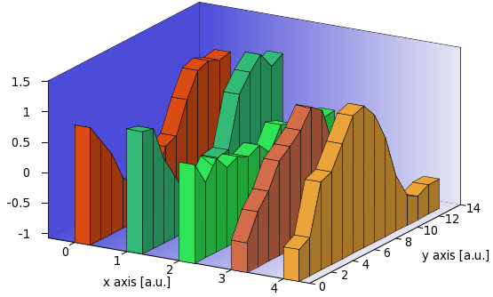
I believe, there is not too much else that we could do here, but we have gone a long way, and produced a decent-looking wall chart! I should also point out that, if you want to use the second plot, i.e., the wall chart without the roofs, you can still add a grid. All you have to do is to add those three lines that we discussed in connection with the grid on the complete wall chart.